
Dimensionalities
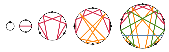
The idea of using other-than-Cartesian coordinates came to me while out for a walk. For years I’d been fascinated by Buckminster Fuller, particularly his interest in the Platonic solids, along with what he named the “vector equilibrium” (VE). I saw that there were ways of identifying points within frameworks other than the orthogonal (right-angle relation) axes used in Cartesian coordinates. I then saw that there were also non-Cartesian ways of identifying points in 1 and 2 dimensions.
(10/23/23) I’m going to introduce aspects of this differently than before. Presume there is a “measure twice, cut once” aspect to accuracy/precision of an observation. So I will discuss frameworks that can be used to measure/identify something’s location – along a line, on a plane, in a volume. Along a line, if one measures opposite directions from an origin, any point’s coordinates will be (a, -a). The coordinates add to zero. Metaphorically, this could be like measuring profit and the costs somewhere for that profit to exist. Just measuring in one direction could be seen as a “good enough” shortcut. This method of finding balance can be extended to have axes pointing to x, -x, also y, -y in a plane, and z, -z in a volume.
In a plane, three axes can be arranged so that coordinates add to zero. There’s a diagram below in my earlier descriptions. From the center of a triangle, form 3 axes in the directions of the corners of the triangle. The diagram demonstrates the 3 coordinates adding to zero. This form of adding to zero can be extended for volumes by forming axes whose + and – directions point to the vertices of a cuboctahedron, what Bucky Fuller called a Vector Equilibrium (or VE). One way of imagining the shape is by nesting a cube and an octahedron – with the center points of the edges of one touching the center points of the edges of the other. The VE is the volume in common. The six +/- axes have four subsets of 3 axes that form planes where the coordinates add to zero. However, I don’t think it’s possible to assign + and – directions to each of the pairs that will work in all 4 planes.
In a volume, there is a way to arrange four axes so that the coordinates add to zero. From the center of a tetrahedron, form 4 axes in the directions of the vertices of the tetrahedron.
The convention I use to name an axis system is xMy where x is the number of axes and y the number of dimensions being measured. Cartesian coordinates are 1M1, 2M2, and 3M3 in 1, 2, or 3 dimensions. Including the mirror-image (opposite direction) for each of these form 2M1, 4M2 and 6(0)M3. There are three different axis systems that use 6 axes to measure 3 dimensions, so I use 6(0)M3, 6(1)M3, and 6(2)M3 to distinguish them.
The tetrahedron, octahedron, cube and VE can all be oriented to the 3M3 (the x/y/z Cartesian coordinates we’re used to), 4M3 and 6(1)M3 coordinate systems. The icosahedron and dodecahedron can both be oriented to the 6(2)M3, 10M3 and 15M3 coordinate systems.
Geometric relationships in the Coordinate Systems
The 3M3 and 6(0)M3 coordinate systems (Cartesian x,y,z) appear in the vectors from the
- center of a tetrahedron to the centers of its edges
- center of an octahedron to its vertices
- center of a cube to the centers of its faces
- center of a VE to the centers of its square faces
The 4M3 coordinate system (4 coordinates that sum to zero) appears in the vectors from the
- center of a tetrahedron to its vertices (negative direction is to the centers of its faces)
- center of an octahedron to the centers of its faces
- center of a cube to its vertices
- center of a VE to the centers of its triangular faces
The 6(1)M3 coordinate system (6 coordinates, out of which 4 sets of 3 form 3M2 coordinate planes) appears in the vectors from the
- center of an octahedron to the centers of its edges
- center of a cube to the centers of its edges
- center of a VE to its vertices
Planes perpendicular to the axes of the 4M3 coordinate system are where the 3M2 subsets of 6(1)M3, as mentioned above, occur.
The relationship between 6(1)M3 and 6(2)M3 is interesting. If you take two opposite corners of any one of the square faces of a VE and pull them together (or push them apart) so that the square becomes two triangles (either change will echo in the other 5 squares), you get an icosahedron (with 20 triangular faces).
The 6(2)M3 coordinate system appears in the vectors from the
- center of of an icosahedron to its vertices
- center of a dodecahedron to the centers of its faces
The 10M3 coordinate system appears in the vectors from the
- center of an icosahedron to the centers of its faces
- center of a dodecahedron to its vertices
The 15M3 coordinate system appears in the vectors from the
- center of either icosahedron or dodecahedron to the centers of its edges – in other words, where the nested shapes touch.
Others’ work closest to mine (that I’ve found) is that of Kirby Urner (who knew and worked with Bucky Fuller) — his Quadrays are similar to my 4M3 (see below). In light of an email exchange with him, I better understand the difference in our outlooks. He is particularly interested in an arrangement of vectors (rather than bi-directional axes) oriented in the same way as 4M3 — Kirby notes that a caltrop has this shape.
There are two aspects of the concepts discussed here that need to be separated in order to show where my approach and Kirby’s are similar, and where they diverge.
The first is, for each dimension (line, plane, space), considering the various arrangements of axes that might be used in that dimension (the xMy arrangements discussed here). Kirby and I are both fond of the “caltrop” (4M3) arrangement of axes, as was Bucky Fuller. Kirby concentrates almost exclusively on the 4M3 axis-pattern. I’m looking to see that as one of many of the coordinate systems possible via the structures of the Platonic Solids, and how these alternate coordinate systems inter-relate.
The second is, for each of the axes in a given set, how, mathematically, the axis is used. I use number lines with coordinates extending from negative to positive infinity. Kirby uses vectors (hence the “ray” in Quadray) with non-negative magnitudes. Where I go into a “sums to zero” property of some coordinate systems, there is a related property in Kirby’s Quadrays. He shows that one can get to any point in a 3-dimensional space by going only positive distances in at most 3 of the 4 directions of the “caltrop”.
Zero-balanced coordinates
Cartesian coordinates give the minimum amount of information to identify a location. An interesting property of the coordinate systems 2M1, 3M2 and 4M3 is that the values along the axes, when added together, sum to zero. That means there’s a sort of built-in error-checking. As well, all have the property Kirby discusses, of non-negative vectors covering the relevant space.
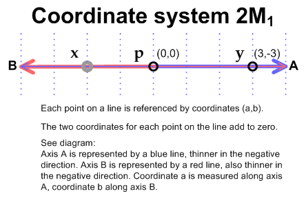
In One Dimension
2M1 is simply a standard Cartesian single dimension paired with its mirror opposite. Point X has coordinates (-2,2).
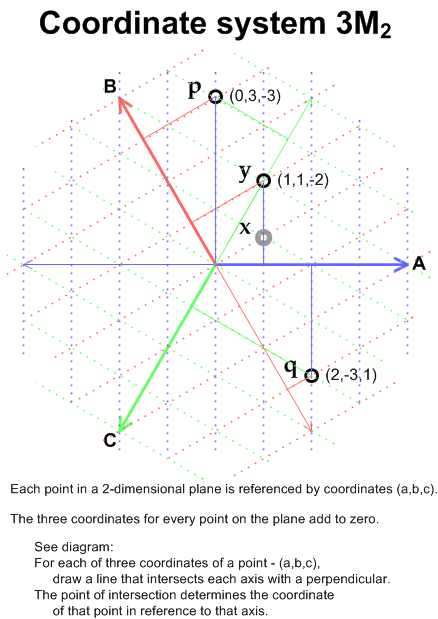
In Two Dimensions
In addition to Cartesian-aligned 2M2 and 4M2 is 3M2, a Zero-balanced system in two dimensions using three coordinates (shown in the image below). 3M2 has 3 axes oriented on a plane from the center of a triangle towards its three corners (or towards the centers of its three sides). Coordinates (a,b,c) are given in the diagram below for points p, q, and y. Point x is precisely between p and q – hence, its coordinates can be determined by averaging the coordinates of p (0,3,-3) and q (2,-3,1) to get (1,0,-1) for x.
In Three Dimensions
4M3 has 4 axes oriented in 3D space from the center of a tetrahedron to its four vertices (or towards the centers of its four faces). No diagram here (for now) – see Quadrays or Google caltrop.
4M3 is a connecting point between Kirby’s ideas and mine. I haven’t seen him discuss applying the properties of the Quadray to a plane (2D vs 3D). He does talk a bit about the “BiRay” (though he doesn’t use that term) – needing two vectors in opposite directions to cover the 1D space.
Beyond Three Dimensions
My intuition tells me (but it is beyond my visualization capacity) that there are similar coordinate systems (where the measure of all the axes sum to zero) in higher dimensions – 5M4, 6M5 and so on. The sequence can be described easily – pull the center point in a direction perpendicular to all the existing axes, to get a symmetric pattern in the next higher dimension. Pull the center point two axes in opposite directions (2M1) to get three axes pointing to the corners of a triangle (3M2). Pull its center point to get axes pointing to the corners of a tetrahedron (4M3), and so forth.
Non-Zero Balanced in Three Dimensions
When Bucky talked about the Platonic solids, he often also discussed the cuboctahedron which he called the Vector Equilibrium (or VE). It’s formed by the (space enclosed by the) points at the centers of the edges of either the cube or the octahedron. (Another way of saying this is, the points where the edges of a nested cube and octahedron touch). It’s closely tied to 6(1)M3.
There are three different versions of 6M3, which I identify using a subscript to the 6, and which I will write here as 6(0)M3, 6(1)M3 and 6(2)M3. 6(0)M3 is a doubling of 3M3 (same process as with 2M1 and 4M2). 6(1)M3 has axes oriented from the center of a Vector Equilibrium (VE) to its vertices. 6(2)M3 points to the vertices of the icosahedron. The re-orientation of going from 6(1)M3 to 6(2)M3 can be thought of as taking the opposite corners of one of the square faces of the VE and pulling closer until you get two equilateral triangles. Doing all the “matching” pulls across all the other square faces completes the transformation of the VE into an icosahedron.
Mathematical relationships between the Coordinate Systems
I’ve not had a mathematician double-check and OK what I’ve written below, so consider it a draft.
The connection between 3M3‘s (x,y,z) coordinates and 4M3 (let’s use (p,q,r,s) ) is (leaving out a constant conversion factor to “equalize” lengths):
- p=x-y-z,
- q=y-x-z,
- r=z-y-x,
- s=x+y+z.
The connection between 3M3 and 6(1)M3 (let’s use (i,j,k,l,m,n) ) is (leaving out a different conversion factor):
- i=x+y,
- j=x-y,
- k=x+z,
- l=x-z,
- m=y+z,
- n=y-z.
These 4 and 6 vectors each have a negative, e.g., -p=-x+y+z, -i=-x-y.
In sum, the 8 possibilities of combining 1 each of +/-x, +/-y, and +/-z map directly to +/- p,q,r,s. The 12 possibilities of combining any two from the same set (+/-x, +/-y, and +/-z) map directly to +/- i,j,k,l,m,n.
I haven’t tried to work out similar relationships to 6(2)M3, 10M3, or 15M3.
Connections Elsewhere
Fuller gave the name to the Vector Equilibrium because he perceived it to be the shape right at the balance point between being inward focused and outward focused (this is a rough approximation of his idea) – at an equilibrium point between imploding and exploding. The pattern of its edges and the struts between center and vertices ARE an octet truss. Flooring made with an octet truss has some rather interesting engineering attributes – such as the way it distributes a load put at any point on its surface.
Kirby Urner has worked diligently for decades to bring some of Buckminster Fuller’s ideas to a wider audience. He uses the term Quadrays (or Quadray Coordinates) to describe something similar to what I call 4M3. More info on this can be found at http://www.grunch.net/synergetics/quadintro.html or on Wikipedia.